Media Mix Modeling Demo

Load data and look at correlations

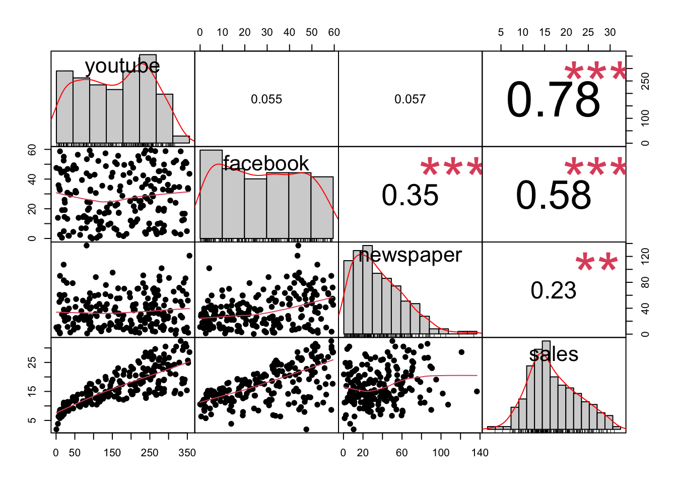
At first glance, youtube and facebook ad budgets seem to be correlated with sales; newspaper spend shows less of a clear relationship.

Adstock adjustment

Because advertising may affect a customer’s behavior for an extended period after exposure, we will adjust the spend amounts per week to include additional amounts from the previous two weeks (adstock). The exact decay rates vary depending on the medium and other factors; here I will use rates of 10%, 15% and 25% for facebook, youtube and newspaper, respectively. All will have a “memory” of two weeks.

The adstocked values are our new predictors (better than raw spend). We are specifying sales as the dependent variable in the lm() function

mmm_1 <- lm(df_sample$sales ~ ads_youtube + ads_fb + ads_news)
summary(mmm_1)

## 
## Call:
## lm(formula = df_sample$sales ~ ads_youtube + ads_fb + ads_news)
## 
## Residuals:
##      Min       1Q   Median       3Q      Max 
## -10.0023  -1.2174   0.3924   1.4328   4.0541 
## 
## Coefficients:
##              Estimate Std. Error t value Pr(>|t|)    
## (Intercept)  1.947558   0.460560   4.229  3.6e-05 ***
## ads_youtube  0.045187   0.001479  30.557  < 2e-16 ***
## ads_fb       0.188177   0.009220  20.410  < 2e-16 ***
## ads_news    -0.005953   0.006041  -0.985    0.326    
## ---
## Signif. codes:  0 '***' 0.001 '**' 0.01 '*' 0.05 '.' 0.1 ' ' 1
## 
## Residual standard error: 2.168 on 196 degrees of freedom
## Multiple R-squared:  0.8819,	Adjusted R-squared:  0.8801 
## F-statistic: 487.9 on 3 and 196 DF,  p-value: < 2.2e-16

There was a small but significant pearson correlation between newspaper and facebook ads in the raw data. Multicolinearity could make it hard to interpret the results, so let’s check for it with a Variance Inflation Factors test:

imcdiag(mmm_1, method = "VIF")

## 
## Call:
## imcdiag(mod = mmm_1, method = "VIF")
## 
## 
##  VIF Multicollinearity Diagnostics
## 
##                VIF detection
## ads_youtube 1.0032         0
## ads_fb      1.1504         0
## ads_news    1.1497         0
## 
## NOTE:  VIF Method Failed to detect multicollinearity
## 
## 
## 0 --> COLLINEARITY is not detected by the test
## 
## ===================================

Fortunately no multicolinearity is detected. Checking for bias and heteroskedacity:

par(mfrow = c(2,2))
plot(mmm_1)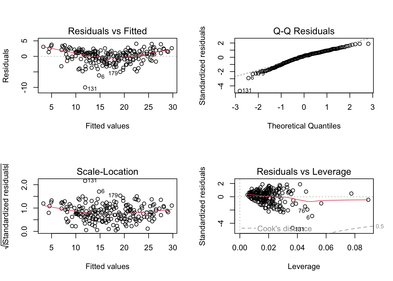

Based on these residuals vs fitted value plots, the residuals are possibly a little biased, but not heteroskedastic. The Breusch-Pagan test confirms this.

lmtest::bptest(mmm_1)

## 
## 	studentized Breusch-Pagan test
## 
## data:  mmm_1
## BP = 4.1583, df = 3, p-value = 0.2449

Add time series element

It’s possible that cyclical seasonal effects (or an overall downward or upward trends) will have more influence on sales than marketing channels. To test this, first we need to add a timeseries variable (just 1:52 repeated over the length of the data; we don’t need to map it to real dates for now). We can decompose this timeseries with the decompose function and see the effect of seasons and trend.

## Add a time series column to investigate trend/seasonality
ts_sales <- ts(df_sample$sales, start = 1, frequency = 52)
ts_sales_comp <- decompose(ts_sales)
plot(ts_sales_comp)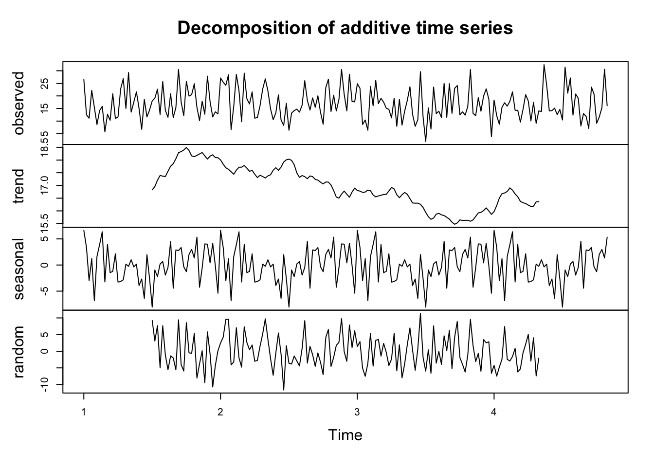

Are these factors significant? Let’s fit another linear model with trend and season added.

mmm_2 <- tslm(ts_sales ~ trend + season + ads_youtube + ads_fb + ads_news)
summary(mmm_2)

## 
## Call:
## tslm(formula = ts_sales ~ trend + season + ads_youtube + ads_fb + 
##     ads_news)
## 
## Residuals:
##     Min      1Q  Median      3Q     Max 
## -6.8701 -1.0978  0.1012  1.1498  5.5102 
## 
## Coefficients:
##              Estimate Std. Error t value Pr(>|t|)    
## (Intercept)  4.550710   1.269482   3.585 0.000461 ***
## trend       -0.001346   0.002698  -0.499 0.618585    
## season2     -2.439879   1.500236  -1.626 0.106066    
## season3     -3.837931   1.511244  -2.540 0.012160 *  
## season4     -0.019777   1.505982  -0.013 0.989540    
## season5     -2.589598   1.533250  -1.689 0.093391 .  
## season6     -2.975709   1.500929  -1.983 0.049317 *  
## season7     -1.828409   1.498110  -1.220 0.224279    
## season8     -1.737503   1.499661  -1.159 0.248538    
## season9     -1.735511   1.542630  -1.125 0.262446    
## season10    -2.379873   1.520560  -1.565 0.119747    
## season11    -3.564521   1.504577  -2.369 0.019158 *  
## season12    -2.221964   1.503207  -1.478 0.141552    
## season13    -2.126054   1.502541  -1.415 0.159235    
## season14    -1.757011   1.537121  -1.143 0.254913    
## season15    -1.008243   1.507831  -0.669 0.504776    
## season16    -0.971702   1.504299  -0.646 0.519340    
## season17    -1.675260   1.510448  -1.109 0.269230    
## season18    -1.487987   1.499527  -0.992 0.322714    
## season19    -3.228179   1.516448  -2.129 0.034975 *  
## season20    -0.920816   1.496122  -0.615 0.539217    
## season21    -2.694057   1.496636  -1.800 0.073942 .  
## season22    -2.724598   1.534971  -1.775 0.078008 .  
## season23    -4.770156   1.513552  -3.152 0.001976 ** 
## season24    -2.457553   1.519227  -1.618 0.107930    
## season25    -0.131696   1.520747  -0.087 0.931110    
## season26    -2.774732   1.523675  -1.821 0.070671 .  
## season27    -5.345331   1.525779  -3.503 0.000612 ***
## season28    -1.525467   1.516993  -1.006 0.316301    
## season29    -3.807714   1.501743  -2.536 0.012295 *  
## season30    -1.881424   1.501888  -1.253 0.212343    
## season31    -2.258311   1.511899  -1.494 0.137444    
## season32    -2.855228   1.502809  -1.900 0.059442 .  
## season33    -2.696570   1.502977  -1.794 0.074887 .  
## season34    -2.413012   1.510219  -1.598 0.112282    
## season35    -2.534971   1.521820  -1.666 0.097937 .  
## season36    -2.044690   1.504609  -1.359 0.176287    
## season37    -0.511780   1.509610  -0.339 0.735092    
## season38    -1.460185   1.502723  -0.972 0.332833    
## season39    -1.605796   1.502239  -1.069 0.286887    
## season40     0.044458   1.530591   0.029 0.976868    
## season41    -0.503530   1.515917  -0.332 0.740250    
## season42    -1.542739   1.511224  -1.021 0.309035    
## season43    -2.440774   1.510239  -1.616 0.108250    
## season44    -2.802112   1.506946  -1.859 0.065002 .  
## season45    -4.075788   1.628560  -2.503 0.013443 *  
## season46    -1.791812   1.624069  -1.103 0.271743    
## season47    -1.542609   1.628470  -0.947 0.345085    
## season48    -1.246402   1.616600  -0.771 0.441969    
## season49    -3.781911   1.643492  -2.301 0.022819 *  
## season50    -1.074279   1.637860  -0.656 0.512933    
## season51    -4.164205   1.645888  -2.530 0.012480 *  
## season52    -3.191509   1.648129  -1.936 0.054772 .  
## ads_youtube  0.044778   0.001669  26.825  < 2e-16 ***
## ads_fb       0.185387   0.010483  17.685  < 2e-16 ***
## ads_news    -0.008845   0.006874  -1.287 0.200297    
## ---
## Signif. codes:  0 '***' 0.001 '**' 0.01 '*' 0.05 '.' 0.1 ' ' 1
## 
## Residual standard error: 2.11 on 144 degrees of freedom
## Multiple R-squared:  0.9178,	Adjusted R-squared:  0.8865 
## F-statistic: 29.25 on 55 and 144 DF,  p-value: < 2.2e-16

A couple of weeks are significant in this model, while overall trend is not. However, for predictive purposes, having 50 coefficients in a model with questionable value seems unnecessary and like it could lead to overfitting and inflated standard errors. I want to use a regularization process to select only the important variables for prediction. I will do this using Lasso (least absolute shrinkage and selection operator)

# Best lambda
best_lambda <- cvfit$lambda.min
print(best_lambda)

## [1] 2.750911

# Coefficients at best lambda
coef(cvfit, s = best_lambda)

## 56 x 1 sparse Matrix of class "dgCMatrix"
##                     s0
## (Intercept) 2.07451978
## ads_youtube 0.04496458
## ads_fb      0.17632122
## ads_news    .         
## week2       .         
## week3       .         
## week4       .         
## week5       .         
## week6       .         
## week7       .         
## week8       .         
## week9       .         
## week10      .         
## week11      .         
## week12      .         
## week13      .         
## week14      .         
## week15      .         
## week16      .         
## week17      .         
## week18      .         
## week19      .         
## week20      .         
## week21      .         
## week22      .         
## week23      .         
## week24      .         
## week25      .         
## week26      .         
## week27      .         
## week28      .         
## week29      .         
## week30      .         
## week31      .         
## week32      .         
## week33      .         
## week34      .         
## week35      .         
## week36      .         
## week37      .         
## week38      .         
## week39      .         
## week40      .         
## week41      .         
## week42      .         
## week43      .         
## week44      .         
## week45      .         
## week46      .         
## week47      .         
## week48      .         
## week49      .         
## week50      .         
## week51      .         
## week52      .         
## trend       .

This shows us that all of the week dummy variables, as well as newspaper spend and trend, have zero coefficients, meaning they do not add predictive power to the model and can be dropped. Lasso penalizes complexity, removing even weakly significant variables if they don’t aid prediction.

# Get nonzero coefficient names (excluding intercept)
lasso_coefs <- coef(cvfit, s = "lambda.min")
selected_vars <- rownames(lasso_coefs)[which(lasso_coefs != 0)]
selected_vars <- setdiff(selected_vars, "(Intercept)")  # exclude intercept
print(selected_vars)

## [1] "ads_youtube" "ads_fb"

Now refit an lm with only the selected variables, Facebook and Youtube spend:

formula_str <- paste("sales ~", paste(selected_vars, collapse = " + "))
formula_ols <- as.formula(formula_str)

# Use the same model matrix columns from df
df_lm <- as.data.frame(X[, selected_vars, drop = FALSE])
df_lm$sales <- y

# Refit OLS
ols_fit <- lm(formula_ols, data = df_lm)
summary(ols_fit)

## 
## Call:
## lm(formula = formula_ols, data = df_lm)
## 
## Residuals:
##     Min      1Q  Median      3Q     Max 
## -9.8037 -1.2752  0.4721  1.4149  4.3137 
## 
## Coefficients:
##             Estimate Std. Error t value Pr(>|t|)    
## (Intercept) 1.770508   0.424036   4.175 4.46e-05 ***
## ads_youtube 0.045147   0.001478  30.544  < 2e-16 ***
## ads_fb      0.184919   0.008606  21.487  < 2e-16 ***
## ---
## Signif. codes:  0 '***' 0.001 '**' 0.01 '*' 0.05 '.' 0.1 ' ' 1
## 
## Residual standard error: 2.168 on 197 degrees of freedom
## Multiple R-squared:  0.8813,	Adjusted R-squared:  0.8801 
## F-statistic: 731.5 on 2 and 197 DF,  p-value: < 2.2e-16

Future predictions

Because our model doesn’t retain any seasonal or trend components as significant, the only factors predicting sales outcome are youtube and facebook spend. Let’s project revenue in the future, adding some noise to weekly spend so as not to get an unrealistically flat line.

fb_mean <- mean(df$facebook) 
fb_sd   <- sd(df$facebook)
yt_mean <- mean(df$youtube)
yt_sd   <- sd(df$youtube)

df_scaled <- df %>%
  mutate(
    fb_spend_scaled = (facebook - fb_mean) / fb_sd,
    yt_spend_scaled = (youtube - yt_mean) / yt_sd
  )

X <- model.matrix(sales ~ fb_spend_scaled + yt_spend_scaled, data = df_scaled)[, -1]
y <- df_scaled$sales

cvfit <- cv.glmnet(X, y, alpha = 1, standardize = FALSE)

# ---  Simulate 100 weeks of time-varying future spend ---

n_future <- 100
future_weeks <- (nrow(df) + 1):(nrow(df) + n_future)

# Simulate using random draws from normal distributions
set.seed(123)
sim_base <- data.frame(
  week = future_weeks,
  fb_spend = rnorm(n_future, mean = fb_mean, sd = fb_sd),
  yt_spend = rnorm(n_future, mean = yt_mean, sd = yt_sd),
  scenario = "Forecast (Baseline Spend)"
)

# Reallocation: +50% facebook spend
sim_realloc <- sim_base
sim_realloc$fb_spend <- sim_realloc$fb_spend * 1.5
sim_realloc$scenario <- "Forecast (+50% Facebook)"

Scale simulated data using historical scaling

scale_future <- function(data, fb_mean, fb_sd, yt_mean, yt_sd) {
  data %>%
    mutate(
      fb_spend_scaled = (.data$fb_spend - fb_mean) / fb_sd,
      yt_spend_scaled = (.data$yt_spend - yt_mean) / yt_sd
    )
}

sim_base_scaled <- scale_future(data = sim_base, fb_mean, fb_sd, yt_mean, yt_sd)
sim_realloc_scaled <- scale_future(data = sim_realloc, fb_mean, fb_sd, yt_mean, yt_sd)

X_base <- model.matrix(~ fb_spend_scaled + yt_spend_scaled, data = sim_base_scaled)[, -1]
X_realloc <- model.matrix(~ fb_spend_scaled + yt_spend_scaled, data = sim_realloc_scaled)[, -1]

# --- Predict sales using Lasso model ---

sim_base$predicted_sales <- predict(cvfit, newx = X_base, s = "lambda.min")
sim_realloc$predicted_sales <- predict(cvfit, newx = X_realloc, s = "lambda.min")

# --- Combine with historical data for plotting ---

df$scenario <- "Actual"
df$week <- 1:nrow(df)
df$predicted_sales <- predict(cvfit, newx = X, s = "lambda.min")

plot_data <- bind_rows(
  df %>% select(week, predicted_sales, scenario),
  sim_base %>% select(week, predicted_sales, scenario),
  sim_realloc %>% select(week, predicted_sales, scenario)
)

## [1] "Forecast sales with no Increase: $16623.31"

## [1] "Forecast sales with +50% Facebook spend: $16773.45"

## [1] "Return on Increase: $150.14"

## [1] "Cost of increased Facebook spend: $4520.3"

So, this doesn’t seem like a good ROI based on this simple simulation. A more realistic next step would be to include a capped budget and include the savings of reallocating, for example, all newspaper budget to Facebook and YouTube.

References

Using R to Build a Simple Marketing Mix Model (MMM) and Make Predictions | Towards Data Science https://towardsdatascience.com/building-a-marketing-mix-model-in-r-3a7004d21239/
Kassambara A (2019). datarium: Data Bank for Statistical Analysis and Visualization. R package version 0.1.0.999, https://github.com/kassambara/datarium.